CClust: Clustering Categorical Datasets

R Package Version 0.0.0.9

2019-11-17

Introduction

CClust is an R package developed to help with clustering categorical datasets. The package can be installed from GitHub using devtools and then loaded in the usual way.

# Installs redres from GitHub
devtools::install_github("yudizhangzyd/CClust")

# Loads the package
library(CClust)

Overview

There are two main functions kmodes and khaplotype coded for clsutering categorical datasets, specifically the khaplotype function in this package can be used on clustering amplicon datasets with quality scores. In both kmodes and khaplotype, three k-means algorithms (Lloyd’s; MacQueen’s; Hartigan and Wong’s algorithm) were adapted to do clustering.

Package Structure

CClust is structured so the available functions fall under one of four categories.

1. Read data: The first manner in which CClust can be used is to obtain NGS datasets from a fastq(a) file. This is done using the function read_fastq to extract and return a list of data information: reads, quality scores and dimension of data. And read_fastq to extract and return a list of data information: reads and dimension of data.

2. Simulate data: The second way to utilize CClust is to is to Simulate clustered categorical datasets. This is done using the function simulator to simulate clustered categorical datasets by using continous time Marcov chain.

3. Clustering: The third way to utilize CClust is to clustering categorical datasets using the following functions.

-khaplotype: Clustering the amplicon datasets with quality scores, only random initialization is avaiable in khaplotype.

-kmodes: Clustering categorical datasets without quality information of the data, different from function khaplotype, it has six different random initialization methods.

4. Evaluation: Lastly, CClust can be employed to evaluate the clustering result by the following functions.

-ARI: Computing the Adjusted Rand Index (Hubert and Arabie 1985) with the use of function adjustedRandIndex in package mclust.

-plot_cluster: Visulizing the clustering results with the use of function dapc in the package adegenet.

This vignette is set up to mimic the package structure. The sections after the introduction are dedicated to one of the three package uses. Additional details on the functions are included in these sections along with explanations of how to interpret the output and examples.

Algorithms

Since both kmodes and khaplotype adapted three k-means algorithms (Lloyd’s; MacQueen’s; Hartigan and Wong’s algorithm), a brief review of these three algorithms are included here.

1. Lloyd’s algorithm (Lloyd 1982)

Lloyd’s algorithm prescribes alternating updates of the centers with updates of the cluster assignments. The algorithm is terminated if no obseravtion is transfered after a full circle of observations.

2. MacQueen’s algorithm (MacQueen 1967)

MacQueen suggested a slight modification on Lloyd’s algorithm: update the affected centers after every change to the cluster assignments. The algorithm is terminated if no obseravtion is transfered after a full circle of observations.

3. Hartigan and Wong’s algorithm (Huang 1997)

Hartigan’s algorithm improves on Lloyd’s and MacQueen’s algorithms by only assigning the observation to a new cluster if the objective function is guaranteed to improve. In particular, it takes into account any change in centers that will occur as a result of the move and makes sure that, even with this change, the value of the objective function will still be improved. Hartigan and Wong additionally define a live set to decide when to terminate the algorithm and to avoid unnecessary calculations. A cluster is no longer a live set only after a full cycle of the observations is made and none of them moved to or from that cluster.

Initialization methods

For function khaplotype, only random initialization is implemented, users can set different seed.

For function kmodes, except for random initialization, there are 5 more initialization methods.

1. H97_RANDOM

The first of two initialization schemes proposed by Huang (1997) uses the first K observations as the initial modes. This initialization scheme is randomized in the R package klaR by selecting K distinct modes at random from the n observations.

2. HD17

Huang (1997) mentioned above interpretted by Python author de Vos (2017).

3. CLB09_RANDOM

A deterministic initialization scheme peoposed by Cao, Liang, and Bai (2009).

4. K-means++

The k-means++ initialization scheme for k-means Arthur and Vassilvitskii (2007) adapted to k-modes.

5. Greedy K-means++

A greedy version of the algorithm mentioned above Arthur and Vassilvitskii (2007).

Example Data

CCluster contains three datasets, which will be used to demonstrate the functions in this vignette.

1. The zoo.int.data dataset is from the UCI Machine Learning Repository (Lichman. 2013). It includes one numeric coordinate, number of legs, which is treated as categorical.

2. The sim.fastq dataset is sampled from a subset of an amplicon dataset mentioned in the paper DADA2 (Callahan et al. 2016). Accordingly, the assignment.txt is the true assignment of that simulation data.

3. The sim.fasta dataset is sampled from a subset of HMP Mock dataset mentioned in the paper DADA2 (Callahan et al. 2016).

4. The sim_small.fastq dataset is a smaller simulated amplicon dataset from the same source mentioned above, it is for demonstrating the use of plot_cluster.

Read data

Fastq File

One of the ways to utilize CClust is to read the FASTQ file. This can be done using the function in the package named read_fastq.

Input

• datafile: Path to a fastq file.

Output

• Return a list contains reads, quality socres (encoded using ASCII 33 to 126) (if read in a fastq file) and the dim of the data.

Functionality

The code below demonstrates the use of read_fastq.

# Read the sim.fastq file
datFile <- system.file("extdata", "sim.fastq", package = "CClust")
dat <- read_fastq(datafile = datFile)
#> Minimum quality score: ( (40)
#> Maximum quality score: G (71)
#> Minimum read length: 251
#> Maximum read length: 251

# Prints the head of the data
dat$reads[1:3, 1:10]
#>      [,1] [,2] [,3] [,4] [,5] [,6] [,7] [,8] [,9] [,10]
#> [1,] "C"  "T"  "T"  "G"  "C"  "T"  "T"  "A"  "C"  "C"  
#> [2,] "C"  "T"  "T"  "G"  "C"  "T"  "T"  "A"  "C"  "C"  
#> [3,] "C"  "T"  "T"  "G"  "C"  "T"  "T"  "A"  "C"  "C"
dat$quality[1:3, 1:10]
#>      [,1] [,2] [,3] [,4] [,5] [,6] [,7] [,8] [,9] [,10]
#> [1,]   67   67   67   67   67   71   71   71   71    68
#> [2,]   67   67   67   67   67   71   71   71   71    71
#> [3,]   67   67   67   67   67   69   71   71   71    71
dat$dim
#> [1] 10000   251

Fasta File

Read a FASTA file.

Input

• datafile: Path to a fasta file.

Output

• Return a list contains reads and the dim of the data.

Functionality

The code below demonstrates the use of read_fasta.

# Read the sim.fastq file
datFile <- system.file("extdata", "sim.fasta", package = "CClust")
dat <- read_fasta(datafile = datFile)
#> Minimum read length: 240
#> Maximum read length: 240

Simulate data

CClust can also be used to simulate clustered categorical datasets. This can be done using the function in the package named simulator.

Usage

Input

• simK Number of clusters.
• n_coordinates Number of coordinate of the simulated dataset.
• n_observations Number of observation of the simulated dataset.
• sim_between_t Between cluster variation.
• sim_within_t Within cluster variation.
• use_dirichlet Indicate if cimulate datasets with dirichlet prior. Defalut is FALSE.
• sim_pi Mixing proportions, a vector with the same length of specified number of clusters and the sum of the values in this vector has to be 1.

Output

• Return a list of simulation dataset results, including the CTMC_probabilities, the true modes, the cluster_assignments, the cluster_sizes and simulated data.

Functionality

The code below demonstrates the use of simulator.

# Simulate data with dim 50 * 5, 4 different categories and there are 5 true clusters.
data <- simulator(simK = 5, n_coordinates = 5, n_observations = 50, n_categories = 4,
sim_between_t = 2, sim_within_t = 1, use_dirichlet = TRUE, sim_pi = c(0.1, 0.1, 0.2, 0.3, 0.3))

head(data$data)
#>      [,1] [,2] [,3] [,4] [,5]
#> [1,]    0    1    2    1    2
#> [2,]    1    1    2    2    0
#> [3,]    2    3    1    2    1
#> [4,]    3    1    2    0    0
#> [5,]    3    1    2    0    0
#> [6,]    3    1    2    0    0

Clustering categorical dataset

CClust has two clustering functions kmodes and khaplotype, kmodes is for clustering categorical datasets without quality information, khaplotype is for clustering datasets with quality information, now it only can be applied to amplicon datasets with quality scores.

kmodes

kmodes is intended to clustering the categorical datasets without quality information, it includes three unsupervised clustering algorithms and six initialization method.

Inputs

• K Number of clusters. Default is 1.
• datafile Path to a data file.
• n_init Number of initializations.
• algorithm Algorithm to implement clustering. The following options are available: -"KMODES_HUANG": MacQueen’s algorithm. (default) -"KMODES_HARTIGAN_WONG": Hartigan and Wong algorithm. -"KMODES_LLOYD": Lloyd’s algorithm.
• init_method Initialization methods. The following options are available: - "KMODES_INIT_RANDOM_SEEDS": Random sampling. (default) - "KMODES_INIT_H97_RANDOM": Huang1997, randomized version. - "KMODES_INIT_HD17": Huang1997 interpretted by Python author de Vos. - "KMODES_INIT_CLB09_RANDOM": Cao2009, randomized version. - "KMODES_INIT_AV07": K-means++ adapted. - "KMODES_INIT_AV07_GREEDY": K-means++ greedy adapted. - ``
• seed Random number seed. Default is 1.
• shuffle Incidate if shuffle the input order. Default is FALSE.

Output

A list of clustering results. The following are returned detials: - "best_cluster_size": Number of observations in each cluster of the best initialization. - "best_criterion": Optimized criterion in each cluster of the best initialization. - "best_cluster_id": Cluster assignment of each observation of the best initialization. - "best_modes": Estimated modes for each cluster of the best initialization. - "best_seed_index": Seed index of the best initialization. - "total_best_criterion": Total optimized criterion of the best initialization. - "clsuter_size": Number of clusters. - "data_dim": Dimension of input data. - "data": The input data.

Functionality

The code below shows how to use kmodes by changing types of algorithms and initialization methods. If run the algorithm more than one initialization, the kmodes function will return results of the initialization with the minimum total_best_criterion, which is the best solution among all of the initializations.

# Clustering with three initializations, default algorithm ("KMODES_HUANG") and shuffel the data with choosing K as 5
datFile <- system.file("extdata", "zoo.int.data", package = "CClust")
res_kmodes <- kmodes(K = 5, datafile = datFile, n_init = 3, shuffle = TRUE)

# Number of observations in each cluster
res_kmodes$best_cluster_size
#> [1] 21 19 23 19 19

# Clustering with Harigan and Wong and K-means++ greedy adapted initialization method.
res_kmodes <- kmodes(K = 5, datafile = datFile, algorithm = "KMODES_HARTIGAN_WONG", init_method = "KMODES_INIT_AV07_GREEDY")

# Mode in each cluster
res_kmodes$best_modes
#>      [,1] [,2] [,3] [,4] [,5] [,6] [,7] [,8] [,9] [,10] [,11] [,12] [,13] [,14]
#> [1,]    0    1    0    0    1    0    0    0    1     1     1     0     0     2
#> [2,]    6    0    0    1    0    0    0    1    0     0     1     0     0     4
#> [3,]    3    0    0    1    0    0    1    1    1     1     0     0     1     0
#> [4,]    0    0    0    0    1    0    1    1    1     1     1     0     1     0
#> [5,]    1    0    1    1    0    1    0    0    0     1     1     0     0     1
#>      [,15] [,16] [,17]
#> [1,]     1     0     1
#> [2,]     0     0     0
#> [3,]     1     0     0
#> [4,]     1     0     1
#> [5,]     1     0     0

khaplotype

khaplotype is intended to clustering the categorical datasets with quality information, now it can be only used on amplicon dataset stored in a fastq file, it includes three unsupervised clustering algorithms and there is only one initialization method: random initialization. khaplotype can also be applied on the datasets that used for kmodes if set run_with_quals = FALSE, however it tends to be slower when implementing Hartigan and Wong’s algorithm.

Inputs

• K Number of clusters. Default is 1.
• datafile Path to a data file.
• n_init Number of initializations.
• algorithm Algorithm to implement clustering. The following options are available: - "FASTQ_LLOYDS_EFFICIENT": Efficient Lloyds algorithm - "FASTQ_HW_EFFICIENT": Efficient Hartigan and Wong algorithm (default) - "FASTQ_MACQUEEN": MacQueen’s algorithm - "FASTQ_LLOYDS": Lloyds algorithm (Same as "FASTQ_LLOYDS_EFFICIENT" but slow, not suggested to use) - "FASTQ_HW": Hartigan and Wong algorithm (Same as "FASTQ_HW_EFFICIENT" but slow, not suggested to use)
• seed Random number seed. Default is 1.
• shuffle Incidate if shuffle the input order. Default is FALSE.
• run_with_quals Indicate if conduct clustering on dataset with quality information. Default is TRUE.

Output

A list of clustering results. The following are returned detials: - "best_cluster_size": Number of observations in each cluster of the best initialization. - "best_criterion": Optimized criterion in each cluster of the best initialization. - "best_cluster_id": Cluster assignment of each observation of the best initialization. - "best_modes": Estimated modes for each cluster of the best initialization. - "total_best_criterion": Total optimized criterion of the best initialization. - "clsuter_size": Number of clusters. - "data_dim": Dimension of input data. - "data": Reads of the input data.

Functionality

The code below shows how to use khaplotype by changing types of algorithms. If run the algorithm more than one initialization, the khaplotype function will return results of the initialization with the maximum total_best_criterion, which is the best solution among all of the initializations.

# Clustering an amplicon dataset and run three initializations with default algorithm ("FASTQ_HW_EFFICIENT")
datFile <- system.file("extdata", "sim.fastq", package = "CClust")
res_khap <- khaplotype(K = 5, datafile = datFile, n_init = 3)
#> Minimum quality score: ( (40)
#> Maximum quality score: G (71)
#> Minimum read length: 251
#> Maximum read length: 251
#> Time cost: 1.050098 secs
#> Log likelihood in 1th initialization: -108539.22 (5 iterations: 2979 4939)
#> Time cost: 0.527932 secs
#> Log likelihood in 2th initialization: -108624.68 (2 iterations: 5074 1)
#> Time cost: 0.790028 secs
#> Log likelihood in 3th initialization: -103563.00 (3 iterations: 2894 577)
#> Time cost is: 2.368182 secs
#> Best optimum is: -103562.999033

# Number of observations in each cluster
res_khap$best_cluster_size
#> [1] 2894  577 1557  200 4772

# The value of objective function of the best solutions
res_khap$total_best_criterion
#> [1] -103563

# Clustering an amplicon dataset and run three initializations with MacQueen's algorithm (shuffle the data)
res_khap <- khaplotype(K = 5, datafile = datFile, n_init = 3, algorithm = "FASTQ_MACQUEEN", shuffle = TRUE, seed = 1)
#> Minimum quality score: ( (40)
#> Maximum quality score: G (71)
#> Minimum read length: 251
#> Maximum read length: 251
#> Time cost: 0.077256 secs
#> Log likelihood in 1th initialization: -197241.29 (2 iterations: 1552 4977)
#> Time cost: 0.060676 secs
#> Log likelihood in 2th initialization: -230540.18 (1 iterations: 4272 5607)
#> Time cost: 0.046734 secs
#> Log likelihood in 3th initialization: -200861.80 (1 iterations: 5070 17)
#> Time cost is: 0.185545 secs
#> Best optimum is: -197241.292293

# Number of observations in each cluster
res_khap$best_cluster_size
#> [1] 1552 4977 2889  571   11

Evaluation

The final way to make use of CClust is to compute the adjusted rand index.

ARI

The function ARI is to compute the adjusted rand index given the estimated assignments and the true assiganments.

Inputs

• est A list of results returned from or .
• truth A numeric or character vector of true assignemts.

Output

• A numberic value between 0 and 1, which indicates agreement between two partitions.

Functionality

The code below shows how to access the clustering results using function ARI.

# Estimate cluster assignments by function `khaplotype`.
datFile <- system.file("extdata", "sim.fastq", package = "CClust")
res_khap <- khaplotype (K = 5, datafile = datFile, n_init = 3)
#> Minimum quality score: ( (40)
#> Maximum quality score: G (71)
#> Minimum read length: 251
#> Maximum read length: 251
#> Time cost: 1.225614 secs
#> Log likelihood in 1th initialization: -108539.22 (5 iterations: 2979 4939)
#> Time cost: 0.634146 secs
#> Log likelihood in 2th initialization: -108624.68 (2 iterations: 5074 1)
#> Time cost: 0.672263 secs
#> Log likelihood in 3th initialization: -103563.00 (3 iterations: 2894 577)
#> Time cost is: 2.532116 secs
#> Best optimum is: -103562.999033
ass <- system.file("extdata", "assignment.txt", package = "CClust")
true_assignments <- as.numeric(read.table(ass, header = F, sep = ""))

# Higher ARI means the similar between two partitions, so the clustering reasults is better
ARI(res_khap, true_assignments)
#> [1] 0.9513036

Plotting

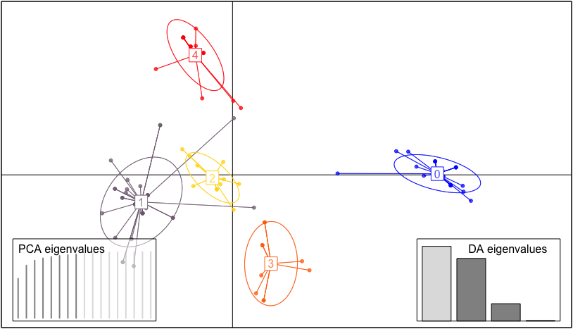
The function plot_cluster helps to visulize clusters after using the cluster algorithms implemented in the functions. This cluster plot make use of the function from package and function from package . The plot is based on observation assignment and discriminant analysis of principal components, therefore, when running the code, it will asks you to choose the number of PCs and the number of discriminant functions to retain.

Inputs

• res Results returned from kmodes or khaplotype.
• xax Integer specifying which principal components should be shown in x axes, default is 1.
• yax Integer specifying which principal components should be shown in y axes, default is 2.
• isGene Indicate if the clustering data is gene sequence.

Output

• A plot reflecting clustering results.

Functionality The code below shows how to plot clusters after running the clustering algorithms using function plot_cluster.

# read the data and use the function `kmodes` with default setting to do the clustering
data <- system.file("extdata", "zoo.int.data", package = "CClust")
res_kmodes <- kmodes(K = 5, datafile = data, algorithm = "KMODES_HARTIGAN_WONG", init_method = "KMODES_INIT_AV07_GREEDY", n_init = 10)

# Plot the clusters
plot_cluster(res_kmodes)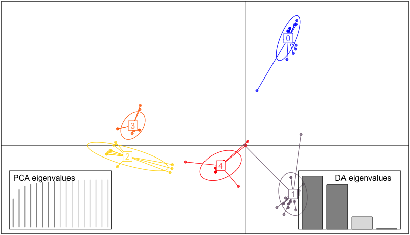

# Plot the clusters by using other principle components
plot_cluster(res_kmodes, xax = 2, yax = 3)

# read the data and use the function `khaplotype` with default setting to do the clustering
data <- system.file("extdata", "sim_small.fastq", package = "CClust")
res_khap <- khaplotype(K = 5, datafile = data, n_init = 10)

# Plot the clusters
plot_cluster(res_khap, isGene = TRUE)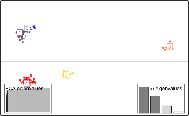

Reference

Arthur, D., and S. Vassilvitskii. 2007. “K-Means++: The Advantages of Careful Seeding. In Proceedings of the Eighteenth Annual Acm-Siam Symposium on Discrete Algorithms, New Orleans, Siam, Pp. 1027-1035.” K-Means++: The Advantages of Careful Seeding, January, 1027–35.

Callahan, B. J., P. J. McMurdie, Michael J Rosen, Andrew W Han, Amy Jo A Johnson, and Susan P Holmes. 2016. “DADA2: High-Resolution Sample Inference from Illumina Amplicon Data.” Nature Methods 13. Nature Publishing Group: 581–83.

Cao, F., J. Liang, and L. Bai. 2009. “A New Initialization Method for Categorical Data Clustering.” Expert Syst. Appl. 36: 10223–8.

Huang, Z. 1997. “A Fast Clustering Algorithm to Cluster Very Large Categorical Data Sets in Data Mining.” Proceedings of the SIGMOD Workshop on Research Issues on Data Mining and Knowledge Discovery 28: 1–8.

Hubert, L., and P. Arabie. 1985. “Comparing Partitions.” Journal of Classification, 193–218.

Lichman., M. 2013. “UCI Machine Learning Repository, 2013.” http://archive.ics.uci.edu/ml.

Lloyd, S. 1982. “Least Squares Quantization in PCM.” Information Theory, IEEE Transactions on 28 (2): 129–37.

MacQueen, J. 1967. “Some Methods for Classification and Analysis of Multivariate Observations.” In Proceedings of the Fifth Berkeley Symposium on Mathematical Statistics and Probability, edited by L. M. Le Cam and J. Neyman, 1:281–97. Berkeley, CA: University of California Press.

Vos, N. de. 2017. “Python K-Modes, Version 0.8.” https://github.com/nicodv/kmodes.